LSTM vs Classical ML for Equity Returns
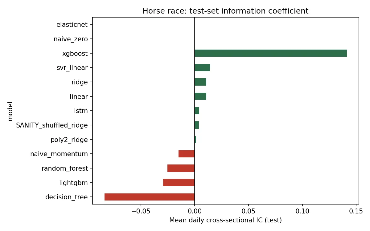
Nothing beats zero on levels; cross-sectionally there is a real stress-regime signal that does not survive transaction costs.
At a glance
- S&P 500 constituents, 2005–2026
- 518
- High-vol cross-sectional IC (t)
- 0.044 (3.2)
- Long-short Sharpe, gross → net
- 2.09 → < 0
- IC at a five-day horizon
- ≈ 0
About this project
An undergraduate research project that benchmarks a pooled-panel PyTorch LSTM against eleven classical models on 518 S&P 500 constituents from March 2005 to July 2026, with a strictly chronological protocol, a shuffled-target leakage alarm that runs on every execution, and a Bloomberg-versus-mirror parity check. After the level horse race returns a null, the task is reframed cross-sectionally and split by a pre-registered volatility regime, with a costed long-short portfolio and a horizon-decay test.
Why it matters
LSTM stock-prediction projects are common and usually wrong for a reason that is invisible in the headline number: leakage, survivorship or an untested baseline. This one is built to fail honestly. The interesting result is what survives the discipline: short-horizon, stress-concentrated cross-sectional predictability that is statistically real and economically useless at the frequencies where it exists.
Methodology
- Panel of 518 S&P 500 constituents exported from a Bloomberg Terminal via a staged VBA export; a yfinance mirror emits the identical schema and was checked against the Bloomberg closes (median absolute difference essentially zero).
- Chronological split only (train to 2021, validation 2022, test 2023+); features from information through the close of day t; scalers fit on train only; a shuffled-target ridge run every time as a leakage alarm.
- Eleven classical models (linear, ridge, elastic-net, polynomial ridge, tree, random forest, XGBoost, LightGBM, linear SVR, two naive baselines) and a pooled-panel LSTM with early stopping. The reported LSTM is the compact configuration (1 layer, hidden 32, dropout 0.1); a higher-capacity 2×64 variant was trained but its test metrics were not retained, so no result is claimed for it.
- Cross-sectional target: each stock’s next-day return minus the equal-weighted universe mean; regime: VIX 63-day z-score > 1, frozen before any test evaluation; decile long-short with turnover and 10 bp per side costs; weekly-rebalance decay test; four-factor risk adjustment.
Strongest findings
- Level prediction: no model beats naive zero on RMSE over 466,426 test stock-days; the LSTM’s test IC is 0.004 (t = 0.76), indistinguishable from the shuffled-target control.
- Cross-sectional, high-volatility days: LightGBM reaches a mean daily rank IC of 0.044 (t = 3.17) versus 0.005 (t = 0.88) on calm days, and the nonlinear model overtakes the linear ones specifically under stress.
- A decile long-short earns a gross annualised Sharpe of 2.09 in high-volatility periods and is negative net of 10 bp per side in every configuration; turnover is roughly 2.7× per day.
- At a weekly rebalance the IC falls to 0.0007: slower trading removes the cost and the edge together. Four-factor alpha is insignificant (t = 1.35 all days, 0.10 high-vol).
Figures
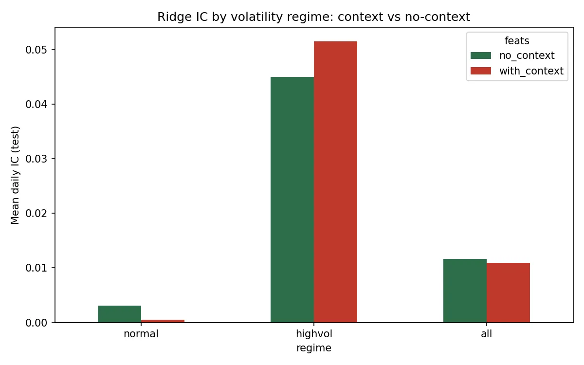
Figure 1. Ridge IC by regime, with and without macro context features: the pooled null hides a high-volatility signal (IC 0.05, t = 3.4). 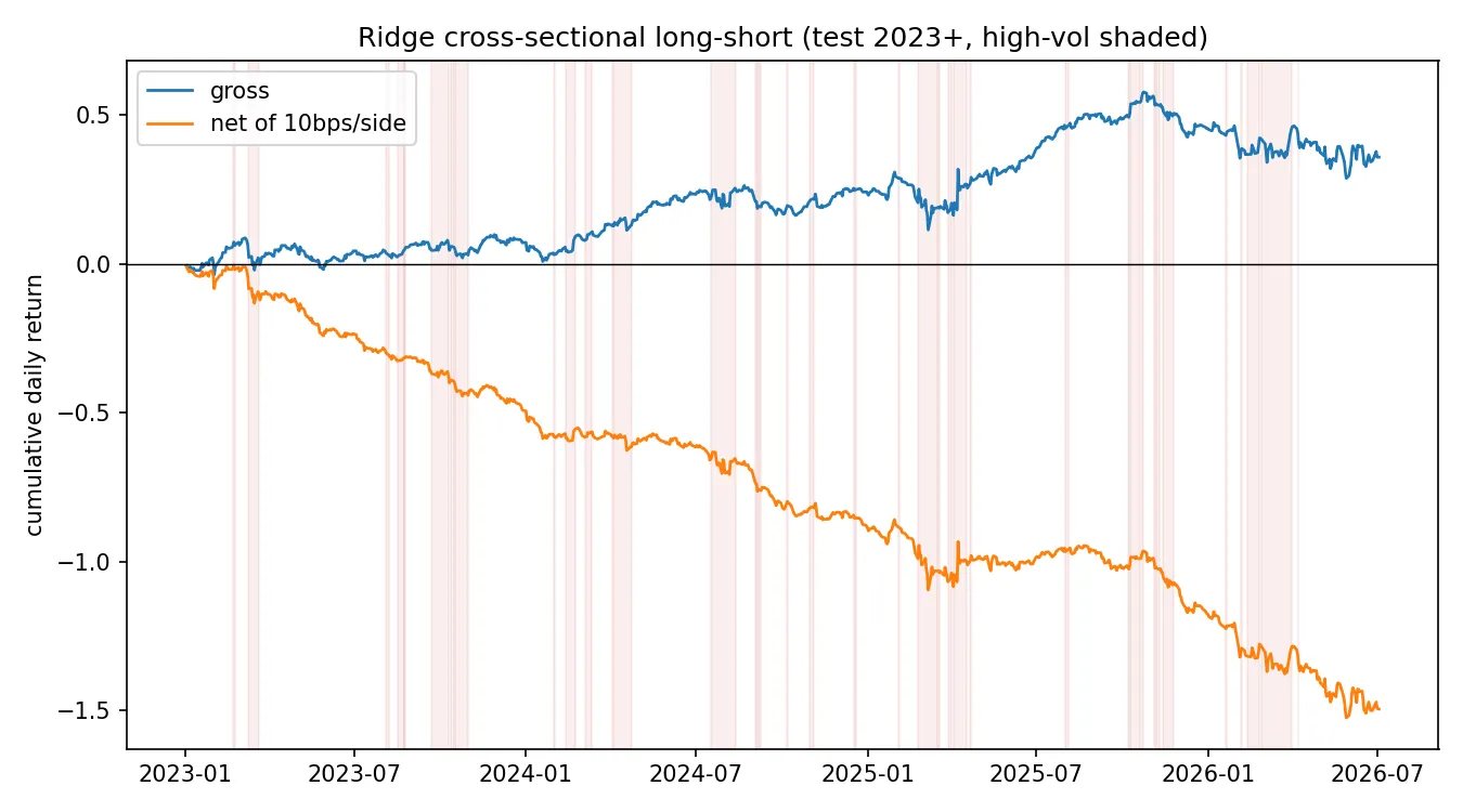
Figure 2. Ridge cross-sectional decile long-short, test period, high-volatility days shaded: positive gross, negative after 10 bp per side.
Robustness and caveats
- Current-member universe, so survivorship bias is present and documented as a limitation.
- Costs modelled as a flat 10 bp per side; one LSTM architecture with four ablations rather than a search.
- The Bloomberg panel and the per-stock prediction files are not redistributed; summary results, checkpoint metrics and the paper are.
- Correction (2026-08-23): the originally typeset paper misprinted the three LightGBM net-Sharpe cells of Table II (−0.24 / −1.91 / −2.02); the correct values are −0.88 / −4.89 / −3.55. The paper served here is the re-typeset, corrected version; the conclusion that every net Sharpe is negative is unaffected.
Challenges
Building a Bloomberg export pipeline that mirrors a free data source exactly, keeping an LSTM honest against a shuffled-target control, and reframing a null into the cross-sectional test that actually answers the economic question.
Learnings
A negative-but-rigorous result is the correct scientific conclusion for this setting. The detectable structure is a one-day, stress-regime phenomenon, and that is exactly where costs are highest.